Snowflake Cortex Analyst: Preventing Join Hallucinations and Double Counting

Navigating complex data schemas is inherently challenging, but it becomes especially difficult in the context of LLM-based text-to-SQL systems. Issues such as fan traps, chasm traps and join path hallucinations are more prevalent, as models are prone to making mistakes or hallucinating. Such errors can lead to problems such as double counting and flawed query logic, fundamentally compromising the trustworthiness of the generated SQL and the insights derived from it.
Snowflake Cortex Analyst’s new ability to support complex schemas flips this narrative. We’re thrilled to announce that we’ve expanded our join capabilities beyond simple star and snowflake schemas to support multifact tables and measures spread across multiple tables — all while maintaining the accuracy of your queries. At the core of this achievement lies a powerful primitive: directed graphs.
In this article, we’ll dive into the challenges of complex schemas, explain how directed graphs enable us to solve them, and show how we use them to prevent join hallucination and double counting.
Representing TPC-H as a granularity graph
First, let’s define a schema to illustrate our solution throughout the article. We’ll use TPC-H, a popular benchmarking data set available by default in all Snowflake account deployments. You can find the data in the SNOWFLAKE_SAMPLE_DATA database.
TPC-H contains all the possible “mines” that make complex joins difficult: multiple join paths, branching directions, multifact table scenarios and converging many-to-one joins at different levels of granularity across eight tables.
One key aspect of our approach is that we represent TPC-H as a “granularity graph”: the backbone of all the algorithms discussed later in this article. This representation has unique characteristics that let us apply our validation logic cleanly.
Our granularity graph is a directed graph where:
Each node corresponds to a unique granularity in our schema. These granularities are not necessarily tied to single tables; a node can merge multiple tables connected by one-to-one relationships as they represent the same granularity.
Directed edges indicate many-to-one joins defined in the semantic model, modeling “projections” toward a higher level of granularity.
Loops (connecting nodes to themselves) each represent a one-to-one relationship.
Here is what the graph representation looks like for TPC-H:
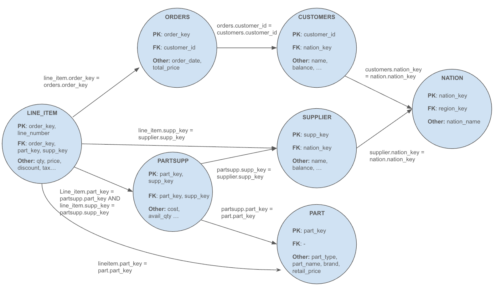
For brevity, we omit some additional annotations that are useful during implementation and keep this diagram focused on the main parts used in this article.
Challenges of complex schemas
To illustrate the problems we’re addressing, consider this example question: What is the total sales and average days outstanding of inventory by part type and nation based on sales from 1997?
A less sophisticated LLM approach without Cortex Analyst might produce SQL like this (notice the commented errors):
WITH sales_1997 AS (
SELECT oli.part_key,
       oli.supplier_key,
       SUM(oli.lineitem_quantity) AS total_quantity_sold,
       SUM(o.total_price) as total_sales_amount --> leads to double counting
FROM order_lineitems AS oli
LEFT JOIN orders AS o ON oli.order_key = o.order_key
WHERE DATE_PART('YEAR', o.order_date) = 1997
GROUP BY oli.part_key,
oli.supplier_key
), part_inventory AS (
   SELECT ps.part_key,
          ps.supplier_key,
          ps.available_quantity,
          p.part_type,
          n.nation_name
   FROM part_suppliers AS ps
   LEFT JOIN parts AS p ON ps.part_key = p.part_key
   LEFT JOIN suppliers AS s ON ps.supplier_key = s.supplier_key
   LEFT JOIN nations AS n ON s.nation_key = n.nation_key
)
SELECT pi.part_type,
       pi.nation_name,
       AVG((available_quantity / NULLIF(total_quantity_sold, 0)) * 365) AS avg_days_outstanding,
       SUM(total_sales_amount) as sales_amount
FROM part_inventory AS pi
LEFT JOIN sales_1997 AS s ON pi.part_key = s.part_key --> missing supplier_key equality
GROUP BY part_type,
         nation_name;
The above queries highlight the two main challenges here: double counting traps and join key hallucinations.
Double counting traps
Double counting occurs when a measure (for example, total_price) is summed multiple times because it appears in repeated rows at a lower-level entity (such as order line items). This inflates totals and yields incorrect results. There are two common pitfalls here, fan traps (like in this example) and chasm traps.
Even experienced SQL writers can slip here: Multitable joins often involve different granularities (for instance, orders vs. line items). If you don’t carefully group or aggregate, each higher-level record (such as an order) gets summed repeatedly for every lower-level record.
With this release, Cortex Analyst is now able to correctly validate against those traps. We will cover the details of how it does it in the last section of this blog.
Join key hallucinations
Join hallucination occurs when the model invents or incorrectly uses a join condition that doesn’t exist in the actual schema and which could cause data errors. This can take two primary forms:
Joins between two tables in the semantic model (easier): When both tables are defined in the semantic model, Cortex Analyst can directly validate the join. If the join in the LLM-generated query matches the user-specified join in the semantic model (for example,
tableA.key = tableB.key) then the join is allowed; otherwise, it’s flagged as invalid and considered hallucinated. Our previous blog post goes into some of the challenges involved in this step.Joins between CTEs (harder): When joining two CTEs in a query, there are no existing join relationships in the semantic model to compare against. In these cases, Cortex Analyst must infer a valid join from the context. Not only that, but it also needs to infer the correct relationship type (many-to-one or one-to-one) between those CTEs to be able to apply validation logic. For instance, if both CTEs are grouped by
part_type, joining on that column might be valid.
In our example query, sales_1997 and part_inventory are both CTEs with no predefined relationship. The query incorrectly joins them only on part_key, omitting the necessary supplier_key. This incomplete join condition causes mismatched rows and ultimately leads to double counting. Without a recognized “table-level” relationship, Cortex Analyst must be able to correctly detect and reject such hallucinations.
Before we go to the solution, let’s define one more important concept using simpler queries.
Finding the granularity node
When writing SQL, we often aggregate data (for example, SUM(), COUNT()) over columns at a specific “level” or granularity. Granularity defines the “uniqueness” of each row. At the orders granularity, each row corresponds to one order. At the customers granularity, each row corresponds to one customer, and so on.
GROUP BY and SELECT DISTINCT are the main SQL constructs that “project” data from a lower granularity (for example, line items) to a higher granularity (for example, orders or customers). For instance, if you query orders and GROUP BY customer_id, your result set effectively has one row per customer. Recognizing this “level” is central to avoiding join hallucinations.
Let’s see how we determine the granularity of a given SQL query.
The algorithm
As described in the section above, each node in our directed graph represents a unique granularity in the schema.
When processing a query, our algorithm:
Identifies all tables (or CTEs) referenced and locates them in the graph
Starts from the most granular node that appears in the query and identifies all possible paths from that node to all leaves
Traverses upward (following many-to-one edges), checking which columns (if any) from the current node appear in
GROUP BYorSELECT DISTINCTStops at the node whose non-foreign-key columns are referenced in the grouping; this node is the query’s granularity
Continues, if only foreign keys are used, up to the next node until a non-foreign-key column appears or until no further nodes remain
Below, we illustrate how this plays out through simple examples.
Example 1: Traversing foreign keys
Consider the following simple query calculating total order amount by customers:
select customer_id,
       sum(total_price)
from orders
group by customer_id
Granularity: customers
Graph traversal:
We start at “Orders,” given it is the only table appearing in the query.
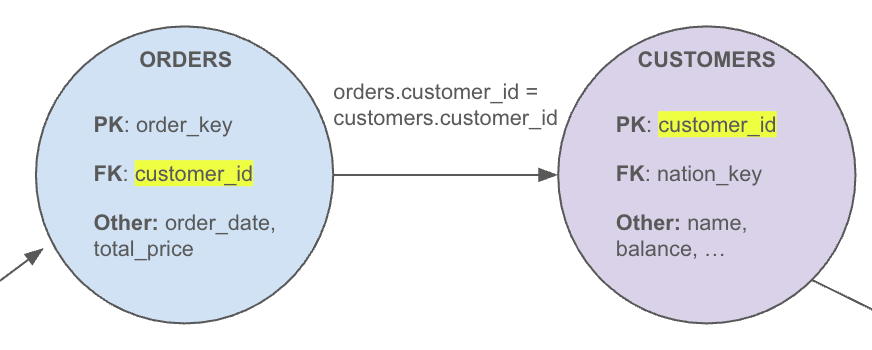
We see that the
GROUP BYuses the foreign keycustomer_id. Since this is not a primary key of “Orders” but does link to “Customers” (without requiring another, unreferenced column in the join path), we move “up” the graph to find the correct granularity level.“Customers” then has its primary key column matching the grouping column
customer_id, meeting our stop criteria in Step 4. So the query’s final granularity is “Customers,” meaning each row of the query output represents a single customer.
This example shows how grouping on a foreign key column can push the granularity up to a different node even if that node is not referenced explicitly in the query. It gets even more complicated when the column name of the foreign key/primary key pair is different on each side of the relationships (for example,orders.customer_id = customers.id), but we will spare you those boring details.
Example 2: Three hop joins
Let’s take this next example answering the question “What is the total quantity per order? Include order date and customer name.”
select o.order_key,
       o.order_date,
       c.customer_name,
       sum(ol.quantity) as quantity
from order_linesitems ol
left join orders o on o.order_key = ol.order_key
left join customers c on o.customer_id = c.customer_id
group by order_key, order_date, customer_name
Granularity: orders
Traversal:
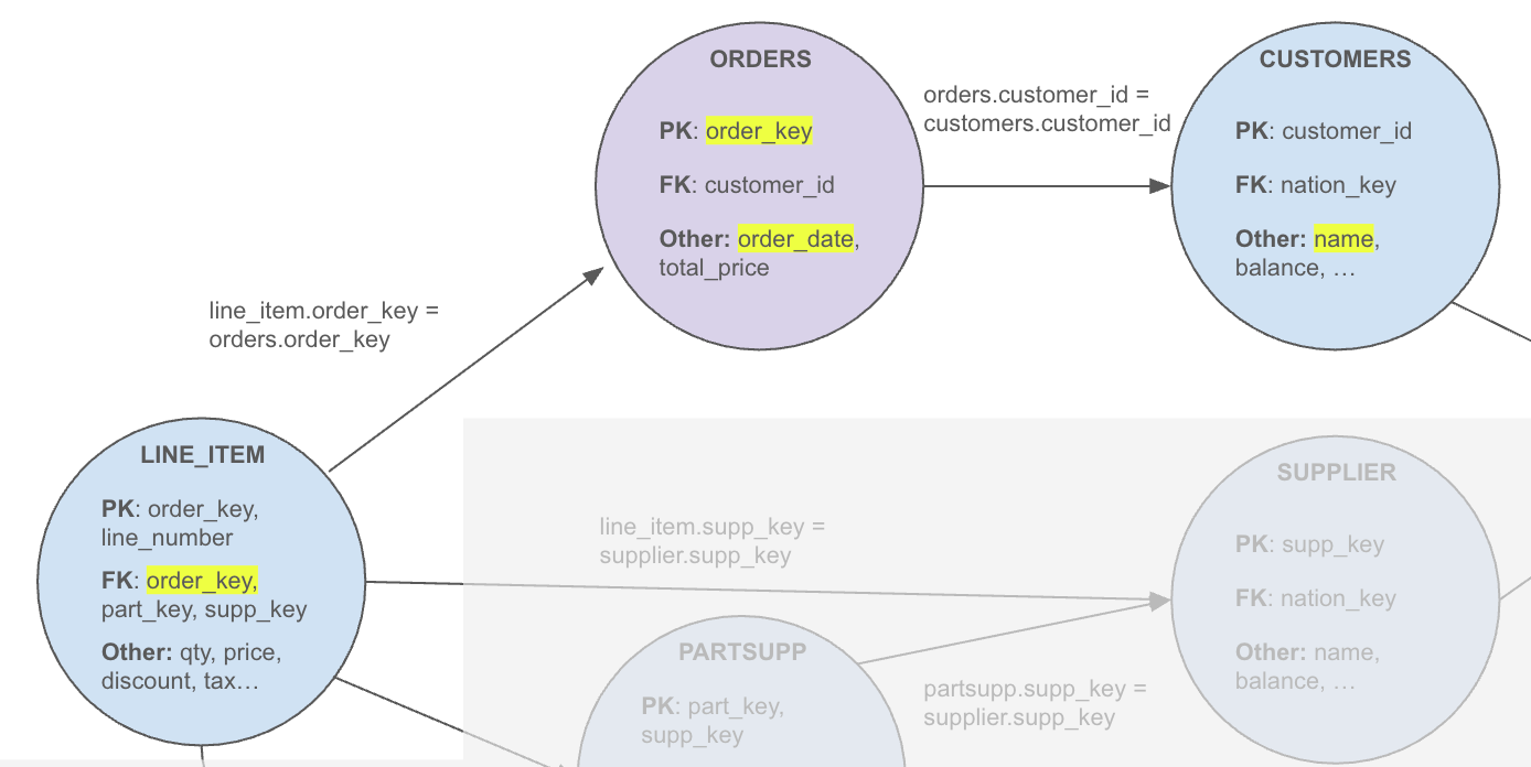
Begin at “Order_Lineitems” as it is the most granular node referenced in the query.
While the GROUP BY references the column order_key in that node, it is a foreign key column so we continue traversal to “Orders.”
Because
order_key and order_dateare non-foreign-key columns of “Orders,” “Orders” is identified as the query’s granularity node. We don’t move further up to “Customers” even though that node is joined in the query and even though the query included customer_name in theGROUP BY.
Example 3: Derived granularity
Now consider a variation representing total quantity by order date and customer name:
SELECT
    oli.order_date,
    c.customer_name,
    SUM(oli.lineitem_quantity) AS total_sold_quantity
FROM order_lineitems AS oli
LEFT JOIN orders AS o
    ON oli.order_key = o.order_key
left join customers c on o.customer_id = c.customer_id
GROUP BY
    o.order_date
In Example 2, we grouped by both order_key (a primary key) and order_date (a normal column) to identify “Orders” as the final granularity node. Here, however, we’re grouping only by order_date. This raises a new question: Is the granularity actually “Orders,” or is it “order_date”?
We call “order_date” a “derived granularity” because:
order_dateis not a foreign key or primary key in the “Orders” node. It’s simply a column that can take identical values across many different orders (for example, all orders placed on 2024-01-01).Conceptually, there is a one-to-many relationship from “order_date” to the actual “Orders” entity because a single date can correspond to many orders.
We don’t yet have a “Date” node for each individual date value because our graph is built around entities (for example, Orders, Customers, Products). Instead,
order_dateis a “derived granularity,” a custom grouping within the “Orders” node.
While this example is good at defining what we mean by “derived,” it does not yet explain why the distinction is useful. In the next section, we will see how derived granularities are handled in queries involving CTEs.
Addressing join hallucinations
Having identified each query’s “granularity” node, we can now tackle join hallucination, where the LLM invents or misuses join paths. Validating these paths is straightforward if the SQL does not involve CTEs or subqueries. When the SQL contains CTEs or subqueries, the join path happens on those derived tables and requires additional work to tie it back to the original join relationship. How do we verify those joins?
A recursive graph-building approach
The solution lies in recursively updating our graph every time we parse a new CTE in the query. Each round looks like this:
Extract all joins from the subquery and validate them against relationships defined in the semantic model
Check whether the join key and join order is correct (details described in this blog post)
If validation errors are encountered, trigger the error correction module (details described in this blog post)
Determine the CTE’s granularity (as described in the previous section)
Examine its source tables, grouping columns and constraints
Identify whether its grouping corresponds to a derived granularity (for example, part type) or an existing entity (for example, parts).
Apply validation logic on the CTE to detect double counting (described in the next section)
Check for fan traps and chasm traps
Trigger the error-correction module if errors are encountered
Add the CTE to the graph, either as a new node or merged with an existing one
If we already have a node at the same granularity, we merge the CTE with that node and insert a self-looping edge to represent an allowed one-to-one join
Otherwise, we create a new node and insert any possible relationships (many-to-one or one-to-many) with previously established nodes
Proceed to the next CTE
Now the context graph has grown. Any future CTE referencing this “freshly minted” node can be validated immediately, as we have established all allowed joins between all entities up to this point.
By the time the final SELECT runs, the graph encodes all necessary relationships, preventing any join that was not validly inferred.
Example joining two CTEs
Consider this SQL snippet, which answers the question “What is the average discount and lowest retail price of each part type?”
WITH discount_per_type AS (
    SELECT
    p.part_type,
    AVG(ol.lineitem_discount) AS avg_discount
    FROM order_lineitems AS ol
    LEFT OUTER JOIN parts AS p
    ON ol.part_key = p.part_key
    GROUP BY
    p.part_type
), lowest_price AS (
    SELECT
    p.part_type,
    MIN(p.part_retail_price) AS lowest_retail_price
    FROM parts AS p
    GROUP BY
    p.part_type
)
SELECT
adppt.part_type,
adppt.avg_discount,
lrpp.lowest_retail_price
FROM discount_per_type AS adppt
LEFT OUTER JOIN lowest_price AS lrpp
ON adppt.part_type = lrpp.part_type
ORDER BY
adppt.part_type;
At first glance, this query introduces two new CTEs, discount_per_type and lowest_price, then joins them on part_type. This join isn’t defined anywhere in the original semantic model, so how do we know it’s valid?
Let’s process each CTE in sequence to verify it.
discount_per_type
The join between "Order_LineItems" and "Orders" is valid as it matches with an edge in our graph.
Grouping by part_type implies a derived granularity from parts given that it is neither a primary key nor a foreign key of the parts table. In this case, we need to create a node for part-type data with a many-to-one link from parts to this node.
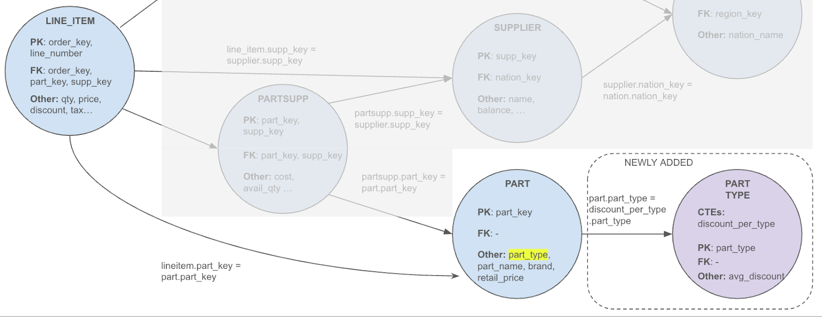
lowest_price
We are not joining any tables here, so we skip the join path validation.
We are again grouping by part_type. This time, the graph already has a node for part-type granularity (the node from the previous CTE), so our final granularity node is part type (and it is not a derived granularity this time).
In this case, we add this CTE to the same node and add a self-loop to represent the one-to-one relationship between them. Additionally, we add a many-to-one join with parts, given that subsequent queries could use that alternative join path.
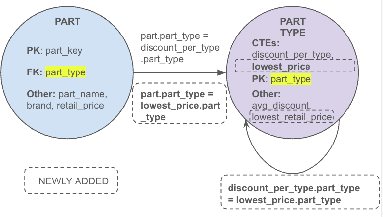
Final SELECT
The join between the two CTEs is matched against the self-loop of the new node. Given that the join tables and keys match the join in the query, it is accepted as valid. If instead the two CTEs were joined, for example, using part_name on one side and part_type on the other, then there would not be an edge in the graph that represents it, flagging it as hallucinated.
This recursive strategy keeps even complex, multi-CTE queries grounded in reality. Instead of allowing arbitrary joins, Cortex Analyst ensures that each step of the SQL, no matter how many derived tables appear, remains faithful to the underlying schema and prevents hallucinated or incorrect relationships.
Eliminating double counting
Now that we’ve seen how join hallucinations are prevented, let’s turn our focus to double counting — a challenge that, once again, hinges on granularity. For every CTE processed during the join-validation step, we also apply double-counting checks using our directed graph. In this phase, we consider only the nodes that appear in the FROM or JOIN clauses, since those are directly tied to how aggregations are applied.
Double counting typically arises from two pitfalls: fan traps and chasm traps.
Fan traps
A fan trap occurs when sequential many-to-one joins create a primary–detail relationship, and the query aggregates measures from both the detail (leaf) table and its immediate primary table.
Consider the following query, which (incorrectly) tries to answer the question, “What is the total quantity and amount sold by customer?”
SELECT
    customer_name,
    SUM(oli.lineitem_quantity) AS total_sold_quantity,
    SUM(o.total_price) as total_price_amount,
FROM order_lineitems AS oli
LEFT JOIN orders AS o
    ON oli.order_key = o.order_key
LEFT JOIN customers c
    ON o.custoer_id = c.customer_id
GROUP BY
    c.customer_name
Here, the total_price measure from the orders table is inadvertently summed for every order line item, inflating the results.
This is what the granularity graph looks like for this query:
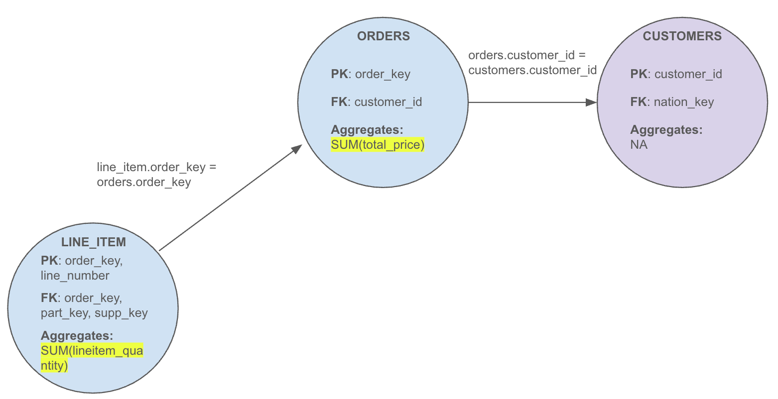
When we represent this query as a granularity graph and annotate each node with its corresponding aggregations, a simple rule emerges: Additive aggregates (e.g., SUM, AVG, COUNT) should only be applied at the lowest granularity node (line_item in this case). In contrast, nonadditive or distinct aggregates (e.g., MIN, MAX, ANY_VALUE) are permitted at any level. If an additive aggregate appears above the root node (like in orders here), a fan trap is detected. One of the benefits of using a granularity graph is that one-to-one relationships are consolidated within a single node, avoiding false positives.
Chasm traps
Chasm traps are more complex and often occur in scenarios involving multiple fact tables. A chasm trap happens when two many-to-one join paths converge on a single table, and the query aggregates measures from both fact tables, resulting in duplicate rows.
For example, consider the question: “What is the total supplier and customer balance by nation?” An incorrect query might look like this:
SELECT
    nation_name,
    SUM(c.customer_balance) as customer_balance,
    SUM(s.supplier_balance) as supplier_balance
FROM CUSTOMERS c
FULL JOIN NATIONS n on c.nation_key = n.nation_key
FULL JOIN SUPPLOERS s on s.nation_key = n.nation_key
GROUP BY nation_name
In this query, the balances are double counted because each customer’s balance is repeated for every matching supplier and vice versa. Let’s look at the subset of the granularity graph representing this query:
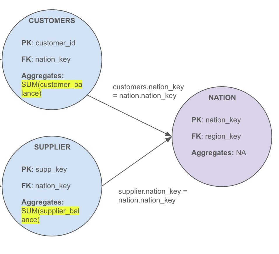
When mapped to a graph, we see three nodes — with two edges converging on the nation node — and both source nodes are contributing aggregated measures. This pattern signals a chasm trap, leading to the query rejection.
A correct approach is to first aggregate each fact table at the appropriate granularity, as demonstrated below:
WITH customer_nation as (
  select nation_key,
         sum(customer_balance) as customer_balance
  from customers
  group by nation_key
) supplier_nation as (
  select nation_key,
         sum(supplier_balance) as supplier_balance
  from suppliers
  group by nation_key
)
SELECT
    nation_name,
    SUM(customer_balance),
    SUM(supplier_balance)
FROM customer_nation c
JOIN NATIONS on c.nation_key = n.nation_key
JOIN supplier_nation s on s.nation_key = n.nation_key
GROUP BY nation_name
By grouping each CTE by nation_key first, both the customer_balance and supplier_balance aggregates are computed at the nation level. Let’s look at the granularity graph representation:
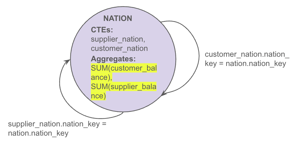
Given the one-to-one relationships between customer_nation, supplier_nation, and nations tables, the final graph for the main SELECT then collapses into a single node, eliminating converging edges and, consequently, signaling no chasm traps and thus, no double counting.
Conclusion
Navigating complex schemas in text-to-SQL LLM systems often leads not only to hallucinated joins but also to double counting issues that can derail query accuracy. Cortex Analyst addresses this by focusing on granularity and representing each entity or derived CTE as a node in a directed graph, while crucially layering robust validation logic on top. This approach ensures that every join is grounded in real relationships, no matter how many derived tables or groupings appear along the way, and actively prevents pitfalls, such as fan traps and chasm traps that result in double counting.
Now that this feature is generally available, we invite you to try Cortex Analyst for yourself. Explore how our graph-based representation and validation logic keep queries aligned with the true schema, helping you unlock reliable insights at scale. Stay tuned for more deep dives into our design and the ongoing enhancements that bring AI-driven SQL to life.
Authors
